Technology

JCMoptimizer comprises many standard tools for the minimization of objective functions CMA-ES, differential evolution or L-BFGS-B. However, often one is faced with expensive functions where these methods are not optimal. Therefore, JCMoptimizer implements a special machine-learning framework that requires far less function evaluations to obtain the same or better results.

Many systems considered in science and engineering exhibit a complex behavior. They are black-box functions in the sense that it is impossible to analytically describe how their output depends on the environmental settings and control parameters. Therefore it is impossible to derive the optimal control parameters for a given objective. Instead one resorts typically to some heuristic optimization approach.

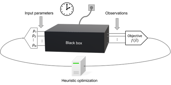
Many heuristic optimization methods rely on a trial-and-error principle. For example, evolutionary algorithms try out new parameter values through mutation and cross-over. While only better parameter values survive, the algorithm does not memorize, what parameter values have been tried in previous generations. Hence, the convergence into a minimum is slow and the whole generation can be trapped in a non-optimal local minimum.

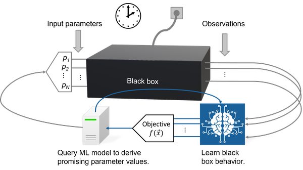
Machine learning (ML) can mitigate the problem of forgetting about previous evaluations of the black box. The ML model tries to learn the dependence of the black box output on the input parameter values. After each evaluation of the black box, the ML model is updated.

The model is queried in order to find promising new parameter values. "Promising" can mean here two different properties:

• The parameter values lead to a convergence into a local minimum of the objective function. This is called exploitation.
• They minimize the uncertainty in parameter space regions with few evaluations. This is called exploration.

Fulfilling only the first point would be easy. One would simply need to find the parameter values for which the ML model predicts the minimal objective value. Evaluation times of ML models are very short such that a global minimization is feasible. However, one could easily get trapped into a local minimum following only this approach.

The second property ensures that ones samples also in new regions of the parameter space. To minimize the uncertainty, it must be known how uncertain the ML model is about its prediction. This information is provided by stochastic ML models. The most common of these stochastic models are Gaussian processes that perform a Bayesian inference on the data of the previous evaluations. This blog entry provides an introduction to Gaussian processes.

Since the optimization uses a stochastic model, if is called Bayesian optimization. Standard Bayesian optimization trains a ML model on the scalar objective value only. We follow a more general approach by learning the higher-dimensional physical output of the black box instead - that is we run a physics-informed Bayesian optimization.

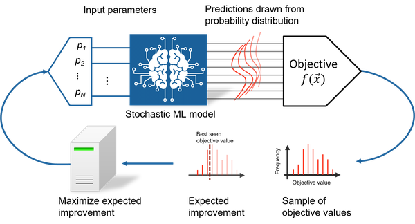
So how can one identify promising parameters, that balance exploitation and exploration? One of the most common strategies is to find parameter values that maximize the expected improvement with respect to the lowest sampled objective value $y_{\rm min}$. The expected improvement is defined as the expectation value $\text{EI} = \mathbb{E}\left[\text{min}(y_{\rm min} - \hat{y},0)\right]$, where $\hat{y}$ is a random variable of possible objective function values.

The expected improvement is large if the mean value of $\hat{y}$ is smaller than $y_{\rm min}$ (exploitation) or if $\hat{y}$ has a large uncertainty such that the lower tail of the probability distribution is smaller than $y_{\rm min}$ (exploration). Due to the balance between exploitation and exploration, the ML model-based approach cannot be trapped in a local minimum and is very sample efficient. More details about Bayesian optimization and a visualization of this behavior is shown in this blog entry.

In the most general case, the JCMoptimizer determines $\text{EI}$ by a Monte-Carlo integration. It does that in a physics-informed way by using information about all black box outputs. That is, it draws a random sample of possible output values from the stochastic ML model. Each vector of output values is mapped to its corresponding objective value, leading to a sample of $N$ objective values $y_1, y_2, \dots, y_N$. These samples are used to estimate $\text{EI}$ as $\text{EI} \approx \frac{1}{N} \sum_{i=1}^{N} \text{min}(y_{\rm min} - y_i,0)$ and to find parameters that maximize $\text{EI}$.

Optimizing a single objective value is only one application. The ML approach implemented into JCMoptimizer is very flexible and allows to run all kinds of studies:

• Often one has multiple objectives and is interested in the trade-off between them (multi-objective optimization).
• While minimizing one objective, there might be also one or more constraints to fulfill. For example, some component of the apparatus should not heat up above a critical temperature (constraint optimization).
• A simulation model of a physical system has some free parameters that should be fit to a set of measurements (model calibration).
• One wants to learn a global model of a complex system, e.g. for the purpose of a global variance analysis (active learning).

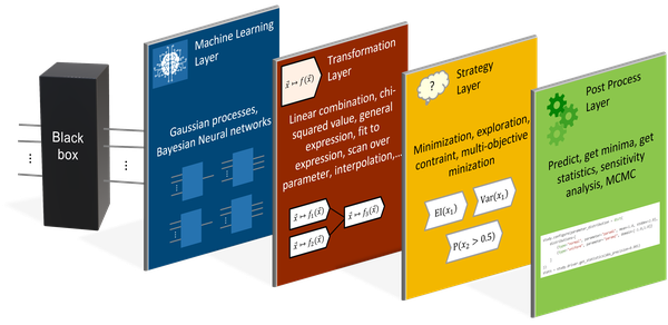
To be applicable in all those scenarios, several layers of the sampling process can be configured independently:

• The machine-learning layer allows to configure one or more ML models.
• The transformation layer maps the output of each ML model to new values.
• The strategy layer defines the sampling strategy.
• After the sampling of the black box is finished, the post process layer enables a further analysis of the system.

The best starting point to learn more about the application areas and the corresponding configuration are our tutorials.